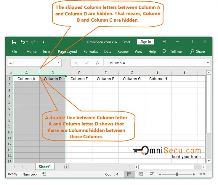
Excel is a powerful tool for organizing and analyzing data, but sometimes worksheets can get hidden unintentionally. When a worksheet is hidden, it can be frustrating trying to find it again. Fortunately, Excel makes it easy to unhide a worksheet with just a few simple steps.
Whether you accidentally hid a worksheet or someone else did, there’s no need to panic. With a few clicks, you can quickly unhide the worksheet and get back to work.
Step 1: Click on the “View” Tab
The first step to unhide a worksheet in Excel is to click on the “View” tab at the top of the Excel window. This tab contains all the options related to viewing and organizing your worksheets.
Step 2: Click on the “Unhide” Option
Once you are on the “View” tab, look for the “Window” group on the ribbon. In this group, you will find the “Unhide” option. Click on this option to see a list of all the hidden worksheets in your workbook.
Step 3: Select the Worksheet to Unhide
After clicking on the “Unhide” option, a pop-up window will appear showing a list of all the hidden worksheets in your workbook. Select the worksheet that you want to unhide by clicking on it, then click “OK.”
Step 4: Confirm Unhiding the Worksheet
Once you have selected the worksheet to unhide and clicked “OK,” the worksheet will be immediately unhidden and visible in your Excel workbook. You can now access and work on the worksheet as usual.
Step 5: Organize your Worksheets
To avoid accidentally hiding worksheets in the future, consider organizing your worksheets by giving them meaningful names and grouping related worksheets together. This will make it easier to navigate through your workbook and minimize the chances of hiding a worksheet unintentionally.
In conclusion, un-hiding a worksheet in Excel is a simple process that can be done in just a few clicks. By following the steps outlined above, you can quickly unhide any hidden worksheet and get back to working on your data analysis. Remember to organize your worksheets to prevent accidentally hiding them in the future.
