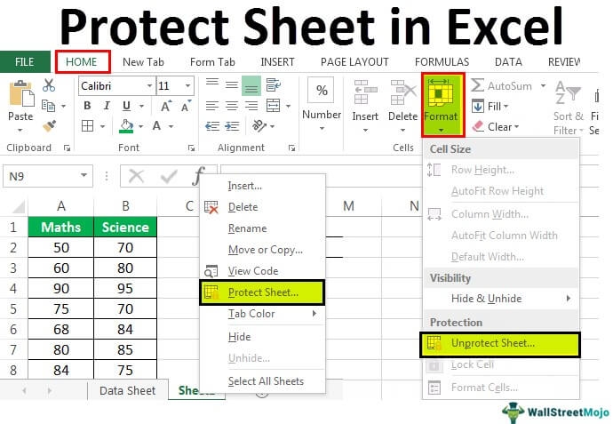
Excel is a powerful tool that allows users to organize and analyze data efficiently. However, it is important to protect the data and formulas in your worksheets to prevent accidental changes or unauthorized access. Fortunately, Excel provides a built-in feature that allows you to protect your worksheets with a password.
By protecting your worksheet, you can ensure that only authorized users can make changes to the data or formulas. This is especially useful when sharing sensitive information or when collaborating on a project with multiple users.
Steps to Protect Worksheet in Excel:
1. Open your Excel workbook and navigate to the worksheet that you want to protect.
2. Click on the “Review” tab in the Excel ribbon at the top of the screen.
3. In the “Changes” group, click on the “Protect Sheet” option. A dialog box will appear with various options for protecting your worksheet.
4. Check the options that you want to apply, such as allowing users to select locked cells, format cells, or insert rows and columns. You can also enter a password to protect the worksheet.
5. Click “OK” to apply the protection to your worksheet. Excel will prompt you to enter a password if you chose to protect the sheet with one.
By following these simple steps, you can protect your worksheet in Excel and ensure the integrity of your data and formulas. Remember to keep your password safe and secure, as it is the key to unlocking the protected worksheet.
In conclusion, protecting your worksheet in Excel is an essential step to safeguarding your data and formulas from unauthorized changes. By utilizing the built-in protection feature, you can control access to your worksheets and maintain the integrity of your work. Follow the steps outlined above to protect your worksheet and enjoy peace of mind knowing that your data is secure.
